


Robustness Beyond Security: An Overview
Origins
In recent years, the study of adversarial examples and robustness had gained great attention, primarily due to the great safety implications. Adversarial examples have the potential to cause crucial ML systems (e.g. self-driving cars) to fail catastrophically with specially manipulated inputs, posing a serious security concern. Fortunately, adversarial training strategies were developed, resulting in “robust” models that are no longer susceptible to these exploits, a great step towards safer Machine Learning.
However, security is only part of the bigger picture - robust models have been found to be much more explainable, manipulable, and intuitive than non-robust classifiers. This was most prominently explored by the Madry Lab in a series of awesome and groundbreaking articles. These newly-found benefits could represent the beginning of an exciting movement towards ML classifiers that not only provide great accuracy, but can also be interacted with in meaningful ways. This post aims to give a simple overview of this advancement in layman’s terms, as well as a graphical example of a MNIST classifier.
What exactly is adversarial training?
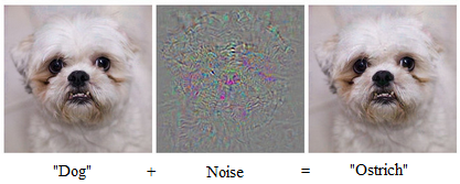
In the context of computer vision classifiers, adversarial examples are images added with a slight but carefully chosen layer of noise, and are barely different from the original image to the human eye. However, the layer of noise causes the model to drastically change its results, and declare the image to be of an entirely different class. Technically, this is mainly due to the model’s “accurate zone” being very narrow - adding even a slight layer of noise causes the image to deviate from the natural images which was model was trained on, and therefore the model reaches a completely incorrect conclusion.
Generating adversarial examples is largely similar to the process of back-propagation. Instead of calculating the partial derivatives of the model’s outputs with regard to the weights, we calculate the partial derivatives w.r.t. the pixels of the input image. We then manipulate the pixels of the input image accordingly, until the output of the model reaches a point we want. In practice, a variety of gradient descent methods and fancy regularization terms could be chosen from to achieve the best results, but the principle is delightfully simple.
To counter this, adversarial training repeatedly generates adversarial examples, and then trains the model on these adversarial examples. In this way, the models learns to be accurate on a “wider” range, and any image that would confuse the model would necessarily look strange to the human eye as well. To put it simply, if someone was to try and confuse an adversarially-trained traffic-sign recognition model with a graphic stuck to a stop sign, then the resulting stop sign would look strange to any humans that see it - clearly a nice feature.
Robustness beyond security
In achieving robustness, models tend to align more with the intuition of human beings, and this is the key towards more manipulable models. At its core, machine learning is still highly statistics-based, and a non-robust model is free to use whatever useful feature it finds. For example, it could well decide that images of a shiny white object with a purely blue background is a plane - because statistically these images do tend to be planes. (This is really just an example - actual features tend to be complex and essentially incomprehensible) However, this is not how humans make the decision - we look for the wings, windows, and engines to decide whether something counts as a plane or not.
The deviation between the model and the human is greatly problematic. Through training on adversarial examples, models are guided to abandon purely statistical features that have no actual meaning, as these fall apart once noise is added. Instead, it resorts to reliable methods of decision that are far more intuitive. (In other words, it’s learning “correlation is not causation” the robot way) With the model’s features aligned with human intuition, it becomes much more manipulable, and potentially yields a variety of uses, such as classifier-based image editing.
Method
To visualize the effects of adversarial training on a model’s manipulability, we perform gradient descent to alter the class of an input image for two MNIST models, one of which is adversarially robust. The two models are otherwise the same, and are based on the CNN classifier from the Tensorflow tutorials. This was done with code strapped onto Madry Lab’s existing mnist challenge repository.
The adversarial training was done with an L2 norm to limit how much each adversarial example may deviate from the original image. In this way, the original label of the image stays true, which is crucial for adversarial training. To satisfy the L2 limit, we use Projected Gradient Descent. In short, PGD conducts a step of gradient descent without regard to the L2 constraint, and then projects the resulting example to the closest example that does satisfy the constraint.
When performing the final class-manipulation on the images, we simply perform gradient descent to maximize the pre-softmax score of the target digit. This is done by calculating the partial derivatives of the pre-softmax score of the target w.r.t. each pixel in the input image, and then manipulating each pixel accordingly.
Results
In large, the robust network displayed much better performance, and traversal to the target class is nearly realistic in some examples. However, performance is inconsistent, and most examples still suffer from large amounts of noise. There is still a long way to go. Manipulating the class does not make for any applications in MNIST, yet the performance here should generalize well to other networks, such as COCO classification, on which traversal between classes could offer many real-world uses.
As seen in the video above, the traversal process is indeed much more successful in the adversarially robust Neural Network (left frame). By frame 130, the traversal had removed the distinguishing features of the number 5, and produced a recognizeable 0, a notable success. The noise became more pronounced as the traversal continued to run, likely because the gradient lacks non-linear terms that allow it to actually converge at a certain point. In comparison, one could argue that the non-robust network produces a very rough 0 by frame 150, but the noise is much more pronounced and random, making the image unrealistic. It is then fair to conclude that adversarial training does have a positive effect on traversal performance, mainly in terms of taming the noise that often appears.
However, the general performance of the robust network is still inconsistent. The level of success heavily depends on factors such as the position of the target image in the frame, the type of digit starting from, and so on. For the videos below, the 2 to 0 transition on the left is able to completely eliminate the 2’s distinguishing features, while the right video largely fails, likely due to the position of the digit. Transitioning to 0 from digits like 5, 6, and 8 works well, while transitioning from 4 to 0 generally produces bad results, since the two digits are not alike to begin with.
Traversal performance clearly has a long way to go, but it has much potential, with changes in architecture and training method possibly bringing further improvements. For example, a certain shortcoming is how adversarial training produces the most effect in a small “radius”: as the original label for each example must stay true, we can only perturb each image so much in adversarial training, and this would only produce the best effect in the initial stages of the traversal.
For further reference, several other random examples from the robust network are displayed below.